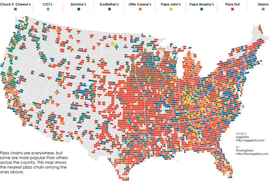
Thematic maps that display data over a surface normally map counts or rates (think census data…dot density, choropleths etc). Nathan Yau isn’t interested in how many pizza restaurants and take-aways there are near to him. He’s interested in how far away the nearest one is so that any order will get to him in the quickest time (road network and traffic allowing of course). Instead, he calculates which pizza chain has the nearest outlet for a grid, calculated as the nearest place within a 10 mile radius across the U.S.

The map creates a fascinating picture not of totality, because having the ‘most’ number of outlets isn’t necessarily optimum for someone wanting to get their dinner in good time, but of relative accessibility. It’s a simple idea but simple ideas often generate interesting work and he brings a good sense of design and a clean graphical approach to the map too.

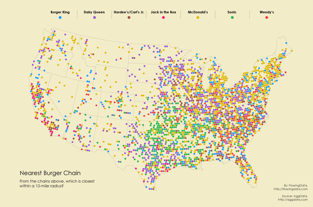
He’s used a similar approach to create a tesselated map of burger joints.

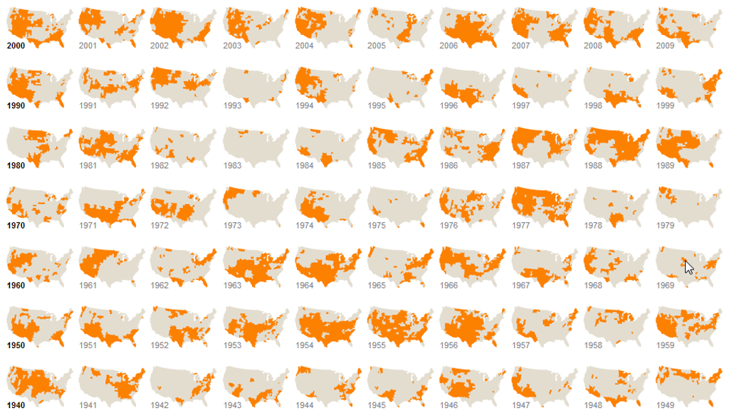
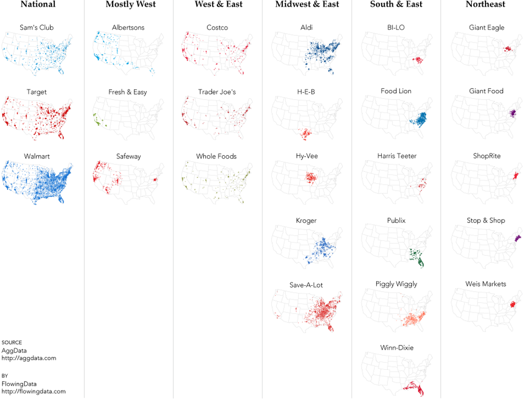
And has also played with small multiples in looking at the spatial preferences of supermarkets.

Exploring datasets using simple thematics is a great way of disentangling the data to eveal particular patterns but these examples show that clear thinking about the specific question you want to answer leads to a clarity in the output too.

There’s more discussion and examples of these maps on Nathan’s FlowingData blog here.

Maps of point based data are all the rage in this open data landscape since most open datasets offer the location of a phenomena by latitude and longitude along with one or more characteristics. Often it’s just a location but that can still reveal insights when analysed and mapped effectively. A data set of all known locations of Starbucks may seem rather tedious because aren’t they on every street corner? Chris Meller took the data and David Yanofsky began mapping it revealing such gems as the location in the USA that is farthest from a Starbucks (Circle, in northeast Montana some 192 miles from the nearest Starbucks). There are 210 locations in Manhattan (slightly more than 6 per square mile) and if you drive from Boston to Philadelphia you’re never more than 10 miles from a Starbucks.

Beyond the factoids, Yanofsky has created some simple yet effective maps to display his findings, such as a map of the USA with a single dot for each Starbucks that pretty much reflects a map of population density. Of more interest here is the small multiples example where he uses a circle of the same size and scale to display the pattern of Starbucks locations in 25 major world cities. The map is well balanced with a 5 x 5 grid of maps. Colours are stark with a Starbuck’s green dot signifying locations against a black background almost like a radar screen.

The map may be simple yet what Yanofsky does he does well. He maintains clarity through symbology, shows a single theme well and uses layout to create a balanced structure. Above all, he is showing comparisons so his maps are each projected properly and use a consistent scale. This is paramount in any mapping application that purports to support visual comparison. Without the correct structure the message can be severely distorted.

Explore a full write-up and more of Yanofsky’s maps in his cartographic guide to Starbuck’s global domination here

Mapping temporal data, particularly to show change, has always been a cartographic conundrum, made all the more difficult the more different time periods you want to show. Animation has often been the standard fallback and is increasingly used in web maps as the technology provides smoother transitions. Of course this approach has one major drawback – you can only see one point in time at any one point in the animation. How, then, do you present data at once to allow visual comparison?

Park and Quealy make excellent use of small multiples here to demonstrate those US Counties classified as under extreme drought conditions from 1896 – 2012. The map forsakes detail which would have demanded a much larger map. It’s not possible to use the maps as a way of looking at counties on an individual basis. The point here, though, is to give clarity and focus to the pattern of change as a general phenomenon and that is achieved to great effect.

While the maps are hosted on a web page, they are static. Adding the ability to mine the data would create a monstrous application that simply isn’t necessary. Each map is two colour; the binary approach is all that is needed so the symbology is stripped to the minimum. An equal area projection ensures areas can be visually compared accurately – important since the map is illustrating areal extent. Each row contains a decade of data, beginning with the start year shown in bold type just to add a little structure and guide the eye.

Small multiples are extremely useful in cartography. This example illustrates why. You can see the online version here.